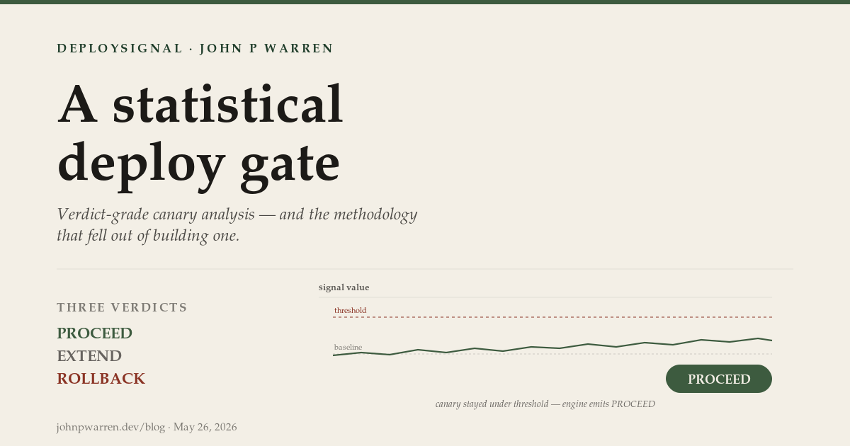
DeploySignal: a statistical deploy gate, and the methodology that fell out of building one
The standard deploy-gate question is also the hardest one in production AI inference: given a deploy and live telemetry, should we proceed, extend, or rollback?
The tools that answer it today — Spinnaker Kayenta, Argo Rollouts, Flagger, Harness Continuous Verification — operate by comparing summary statistics between a canary population and a stable one. They work. They fail in a specific way on AI-inference workloads: regressions in this domain are often multi-modal and slow-developing. A refusal rate creeps up by 6%. A tool-call success rate dips on one cohort. Latency tails widen without the median moving. Each signal stays within its own threshold; the joint pattern is what’s broken. By the time the dashboard alerts fire, the regression has shipped at scale and the rollback is expensive.
DeploySignal answers a narrower version of the same question with statistical rigor: given a stream of multi-signal telemetry from a deploy and its baseline, with formal anytime-valid guarantees on the false-positive rate, fire a verdict. Five detector families run in parallel; each contributes evidence at a different mathematical layer; portfolio fusion produces the decision.
This post is about what DeploySignal is technically, and about what four weeks of building it as a five-role multi-agent project produced as a side effect: the methodology I later published as Anchor, and the engine substrate that Tessera is now built on top of.
The technical core
The deploy-gate problem
A deploy goes out. The dashboard shows green on all the obvious aggregates: p50 latency, error rate, success rate. Over the next several hours, the long-tail behavior degrades — refusal rate climbs gradually, tool-call coherence weakens on a specific tenant tier, a periodic oscillation appears in cache pressure that wasn’t there before. None of these signals exceed their own thresholds. The compound pattern is the regression.
The single-statistic deploy gate is structurally incapable of catching this. It compares one summary to another, computes a p-value or t-statistic, and decides. The class of failure where each signal looks fine in isolation but the joint distribution has shifted is exactly the failure mode that summary-statistic gates miss — by construction.
The narrower question DeploySignal answers: given a continuous telemetry stream and a healthy-baseline reference, can we fire a verdict that holds up under formal anytime-valid guarantees, while catching multi-modal slow-developing regressions that summary-statistic gates miss?
Anytime-valid α and why it matters
Most deploy-gate tools have a fixed α threshold (typically 0.05) and an implicit “check at the end of the canary window” semantics. If you peek mid-window — and operators always peek mid-window — you inflate the false-positive rate. If you don’t peek, you can’t adapt the canary duration based on what the signal is doing.
DeploySignal’s detectors are anytime-valid. The wealth statistic for each family is a supermartingale under the null hypothesis (deploy is healthy). By Ville’s inequality, the probability that the statistic ever crosses a Ville bound during the entire monitoring window is at most α. Operators can read the wealth statistic at every tick without consuming additional α from the budget. The bound holds regardless of stopping rule.
Concretely: an α budget is allocated per family at compile time. Family A gets 40%, Family C gets 20%, Families D and E get 10% each. Family B is rule-based and consumes no α. The total stays within the global budget. Every tick, the audit record tracks α consumption per family.
This is the difference between “you can look once, at the end” and “you can look continuously, and the worst case is bounded.” Operationally, the second is what operators actually want — they want to extend the canary window when the wealth statistic is drifting suggestively but hasn’t crossed, and short-circuit when it has. Anytime-valid is the math that lets you do that without lying about your false-positive rate.
The five detector families
The portfolio is five families running in parallel every tick. Each family contributes evidence under a different statistical model. Any one firing triggers rollback. When multiple families fire on the same event, you get multi-family corroboration — independent statistical tests agreeing.
| Family | Mathematical anchor | Catches | α-budget |
|---|---|---|---|
| A | Page-CUSUM mixture-supermartingale + mSPRT | Per-signal slow drift | 40% |
| B | Hand-tuned structural rules | Known regression archetypes | 0% (rule-based) |
| C | Hotelling T² + Sequential MMD betting e-process | Joint-distribution shift | 20% |
| D | Spectral / autocorrelation + BOCPD | Oscillation patterns | 10% |
| E | Weighted-conformal Mahalanobis novelty | Unknown-unknowns | 10% |
Family A — Per-signal sequential tests. A statistical accumulator that keeps a running tally of log-likelihood-ratio evidence against the healthy hypothesis. Each tick adds evidence; when the accumulator crosses a Ville bound, it fires. Family A catches signals that creep — slow persistent drifts on a single signal that stay below any tick-by-tick threshold but accumulate enough evidence over time to cross the cumulative bound. Six SLIs watched: p99 latency, time-to-first-token, eval score, tool success rate, downstream errors, cost per request. Largest single family in the portfolio.
Family B — Structural signatures. Hand-tuned rules encoding the kind of pattern an experienced SRE would recognize at a glance. The canonical rule is slowbleed: when 4 or more of 9 monitored signals drift in the same direction simultaneously, fire. Each signal’s drift alone is harmless; the synchronized pattern is the architectural signature. Family B is the expert-system layer beneath the statistical ones — rule-based, no α spent, because these are hand-tuned heuristics rather than statistical tests.
Family C — Hotelling T² + Sequential MMD. Multivariate distance from the baseline distribution. Each signal can stay within its own noise band, but if the joint vector sits off the correlation structure that healthy signals normally move along, Family C fires. This is the family that threshold-based systems categorically miss — the regression where each axis looks fine in isolation but the signals are moving wrong relative to each other. Uses Ledoit-Wolf shrinkage on the baseline covariance matrix for numerical stability; Wilson-Hilferty χ² quantile for the threshold. The Sequential MMD component runs as a betting e-process against random Fourier features.
Family D — Spectral / ACF oscillation. Looks for periodic patterns in signals that shouldn’t have them. When a signal starts oscillating — cache flapping, feedback loop, resource cycling — autocorrelation develops a peak at the oscillation lag. Family D sees the peak and fires. A kv_cache oscillating between 60% and 90% every 3 ticks has normal mean and normal variance; its time structure is what’s wrong. Amplitude-based detectors miss this entirely.
Family E — Weighted-conformal Mahalanobis novelty. A nonparametric unknown-unknowns detector. Instead of predicting what failure looks like, Family E compares the incoming deploy vector against a bank of ~16K known-healthy samples. If the new vector is more anomalous than α_E of the calibration samples, it’s flagged — without having to know in advance what went wrong. The other four families assume a model of what degradation looks like; Family E doesn’t.
The design choice across the five is redundancy on purpose. Single-family detectors fail predictably on patterns outside their detection scope. A five-family portfolio with disjoint coverage catches more — and when multiple families fire on the same event, the agreement is itself diagnostic information for the verdict layer.
The calibration compiler
tools/calibrate.ts takes a healthy-baseline trace and produces a CompiledConfig — per-(hour-of-day × day-of-week × tenant-tier) cells, each with its own statistical scaffolding: mean vectors, covariance matrices (Ledoit-Wolf for the parametric path; MCD / MRCD for the robust path), Cholesky factors for fast quadratic-form evaluation, AR(1) phi coefficients for Family A’s drift model, mixture-supermartingale priors, betting-e-process baseline pools for Sequential MMD, conformal calibration scores for Family E.
The compile is deterministic. Same input baseline → same compiled config → same fire decisions on replay. This is the property that makes the system trustworthy as a production deploy gate: when an alert fires, the audit substrate emits a verdict that includes the compiled-config version. Anyone with the same compiled config and the same metric stream can re-derive the same decision exactly.
The tradeoff is heavy upfront, cheap at runtime. The compile takes minutes; runtime is arithmetic against precomputed structures. No matrix factorization at runtime, no threshold recalibration. Per-tick gate-evaluation latency on the full five-family portfolio:
| Scenario | Median | p99 | Max |
|---|---|---|---|
| Healthy path (full evaluation) | 29.8 μs | 62.8 μs | 0.194 ms |
| Regression path (C+E co-fire at t=11) | 27.8 μs | 60.8 μs | 0.167 ms |
For context, a typical LLM token-generation step is 10-100 ms. DeploySignal adds well under 1% overhead on a typical inference-request budget.
The audit substrate
Every detector evaluation emits a structured DetectorVerdict record. Schema sketch:
DetectorVerdict {
  cell_key:           "hour-14_day-tue_tier-bronze",
  baseline_version:   "compiled-config-v4-fusion-novelty",
  schema_continuity:  true,
  family:             "C",
  alpha_consumed:     0.0024,
  alpha_remaining:    0.0476,
  fire:               true,
  fire_reason:        "hotelling_t2_exceeded_ville_bound",
  timestamp:          1714512000.123,
}
These records are replay-clean: same compiled config + same metric stream produces the same verdict. Post-incident reconstruction is exact, not approximate. When an SRE asks “why did the gate fire at 14:23?”, the audit log answers with: which family fired, which cell, how much α was consumed, what the fire reason was, what compiled config was in use. The verdict can be re-derived from first principles.
This is the property that turns DeploySignal from a black-box decision system into something an operator can trust enough to ship behind. The audit record is the contract between the statistical engine and the human who has to defend the rollback decision in the postmortem.
The methodology that emerged
Four weeks, four roles, 250 coordination files
I didn’t set out to invent a methodology. I set out to build DeploySignal. The methodology emerged because the project was statistically nontrivial — the math anchors are multi-paper; the calibration choices are load-bearing in subtle ways; the test coverage has to be rigorous enough that a wrong assumption about how a Cholesky factor is computed turns into a CRITICAL bug that only surfaces under perturbation. Single-pass agent generation produced code that compiled, passed surface-level tests, and would have shipped wrong.
So I structured the work as multi-role: one chat for Architect (the specs), one for Implementer (the code), one for Reviewer (audit), one for TPM (routing between the others) — four agent roles — plus the PM seat, which I held myself. Each role got per-chat project instructions pinning its identity. Coordination state lived in files in a coordination/ directory rather than in chat history.
By around the second week, the directory had 100+ files and patterns started to repeat. The Architect was making the same kinds of attribution mistakes across different topics. The Implementer was committing similar omissions on different specs. The Reviewer was catching the same classes of bug across rounds. Each failure suggested a discipline that, if codified, would have prevented it.
I started writing those disciplines down. By the end of the project, there were about a dozen named disciplines being applied at specific moments in the workflow. The project’s velocity improved measurably — not because the model had gotten better, but because the disciplines were preventing the failure modes that had cost time earlier.
The four weeks produced 250 coordination files, 970 tests, and a reference implementation that passes a reviewer-verified right-reasons audit on 6 canned demos including a reconstruction of a publicly-disclosed AI inference regression. It also produced, as a side effect, a methodology.
What was specifically learned
Three concrete examples — each one a specific moment where a failure produced a discipline that I later named in Anchor.
The Topic 52 phantom chain → memorial accretion. During an investigation of detector behavior on one of the synthetic regressions, an architectural artifact misattributed firing-IDs between the TPR-sweep and FPR-sweep outputs. The Architect built a hypothesis tree on the wrong premise. The chain ran for 7 artifacts before the misattribution was caught via wrapper-bypass log diff. Wall-clock cost: 2-3 days.
The recognition was the moment that mattered. I had a clear memory of similar misattributions happening at least three times earlier in the project — each time resolved as a one-off, nobody had written it down, and so each subsequent occurrence cost the same time to diagnose from scratch. Memorial accretion became a discipline at that point because the same class of failure kept happening and the catalog wasn’t growing to match. From then on, every failure that cost more than half a day got memorialized: what happened, what discipline would have prevented it, where the discipline applies, how its violations and confirmations would be tracked.
The σ² compile-time underflow → the cold-eye Reviewer. 60 of 66 statistical cells were affected by a precision bug in how σ² was computed for bounded-probability features like tool_success_rate and refusal_rate. The bug never surfaced as a test failure during initial implementation — every test the Implementer wrote against the suspect surface passed, because the test fixtures inherited the same precision assumption as the code they were testing.
The Reviewer caught it during an audit aimed at a different question. The recognition: the Implementer cannot audit its own surface effectively, because the tests it writes inherit the assumptions of the code it wrote. The Reviewer’s value is not “second opinion” — it’s “different starting context.” A Reviewer reading the diff cold, with no exposure to the spec rationale or the Implementer’s session history, will notice things the Implementer had no reason to notice. That’s the cold-eye Reviewer discipline.
The wrong-premise architect chain → pre-emit grilling. A spec emitted with a factual claim that wasn’t independently verified (“MCD on the clean fixture produces zero contamination flags”). The Implementer built against the spec; the claim was empirically wrong; the round produced wrong work that the Reviewer caught at audit. Wall-clock cost: 4 days.
The recognition: the most expensive class of error in multi-role work isn’t the implementation bug — it’s the spec-emit-time error that the Implementer absorbs as input. By the time the audit catches it, multiple downstream artifacts have been built on the wrong premise. Pre-emit grilling — adversarial self-review of an artifact before it forwards to the next role — became a discipline because spec-emit-time was where the costliest errors were being made unchecked.
None of these disciplines were known in advance. All of them were learned by failing in a specific way, naming the failure mode, and then naming the discipline that would have prevented it.
The methodology turning around
By the time DeploySignal closed, there were about a dozen named disciplines and a clear sense of which ones were load-bearing (the pack has since grown past fifteen as later projects added their own). I wrote them up as Anchor — disciplines, templates, worked example — and published it as a standalone repo. I hadn’t set out to build a methodology pack; I’d just noticed patterns that seemed like they’d be useful to anyone running multi-role agent work, and writing them up as a pack was the cheapest way to share them.
Then I started Tessera using Anchor from round 1.
The shift was meaningful. DeploySignal’s first 20 rounds had multiple expensive failures of types I now had explicit disciplines for — misattribution chains, self-confirming tests, spec-emit-time errors absorbed as input. Tessera’s first 20 rounds had zero of those failure types. Not because the project was easier — Tessera vendors the DS engine for a different operational scope (per-shard observation of a running cluster), with its own complexity around topology adapters and bi-directional integration contracts — but because the methodology was applied from the start instead of distilled along the way.
Two concrete transfers:
- The audit-trail file discipline transferred directly. Tessera’s
coordination/directory mirrors DeploySignal’s structure: Q-specs, reviewer reports, investigations, dispositions. The shape was already designed. - Memorial accretion transferred with the memorials. Tessera started with about 15 inherited disciplines from DeploySignal that had been paid for in failure. The cross-project memorial file (
~/.claude/CROSS-PROJECT-MEMORIAL.md) is real cross-project capital — disciplines learned on project N applying automatically to project N+1.
The three products together form a lifecycle:
DeploySignal catches before promotion. Tessera observes during steady state. Cairn attributes when something escapes both.
DeploySignal is the pre-promotion gate. Tessera is the steady-state per-shard observer, vendoring the same statistical engine for cluster-scope problems. Cairn is the postmortem attribution layer for incidents that escape both — ranks candidate cause-events against incident onset, closes the loop. Each product applies the methodology to a different operational question; the methodology composes across the three.
Close
DeploySignal is a reference implementation. It isn’t packaged for production deployment as-is — the engine is shipped as runtime-exercised TypeScript modules with a deterministic test substrate, and integration with a specific deployment platform (Argo Rollouts, Flagger, custom Kubernetes operators) is wrap-the-engine work that comes downstream. What it is, instead, is a statistically rigorous answer to a narrowly defined question with provenance guarantees that let an operator replay a verdict and reconstruct the decision exactly.
It is also the project I built before I knew what I was building. The early weeks produced code I’m proud of. The later weeks produced code that’s better than what I would have written without the disciplines that emerged early on. Building something hard reveals the structure of the work in a way that nothing else does. The methodology that emerged exists because the project was statistically demanding enough that single-pass generation didn’t work — and now the methodology applies to other projects because the same constraints hold.
The next post will be about Tessera: what changes when the operational scope is “100-10,000 GPU shards in a running cluster” rather than “one deploy decision,” how the same statistical engine recomposes around per-shard observation, and what 67 rounds of Anchor-methodology development looks like when the disciplines are applied from round 1 rather than distilled along the way.