James Hamilton’s June post on flat datacenter networks reports numbers that should end the fat-tree era: 69% fewer routers, 33% higher throughput, 40% less power, 27% lower operating cost, and a failure curve where losing 1% of routers costs roughly 1% of capacity. The arXiv paper behind it — Bernardi, Mahajan, Seshadhri and colleagues, “RNG: Flat Datacenter Networks at Scale” (arXiv:2604.15261) — reports the design as the new default network for most workloads at Amazon. Then the post and the paper both name the price of all that: paths through a random graph are less predictable than paths through a tree, which makes troubleshooting harder.

That last clause is a fault-localization problem. I had already built a fault localizer — for GPU clusters, not networks — and the question was whether it stayed relevant pointed at a network it was not designed for.

Why the topology stops helping you

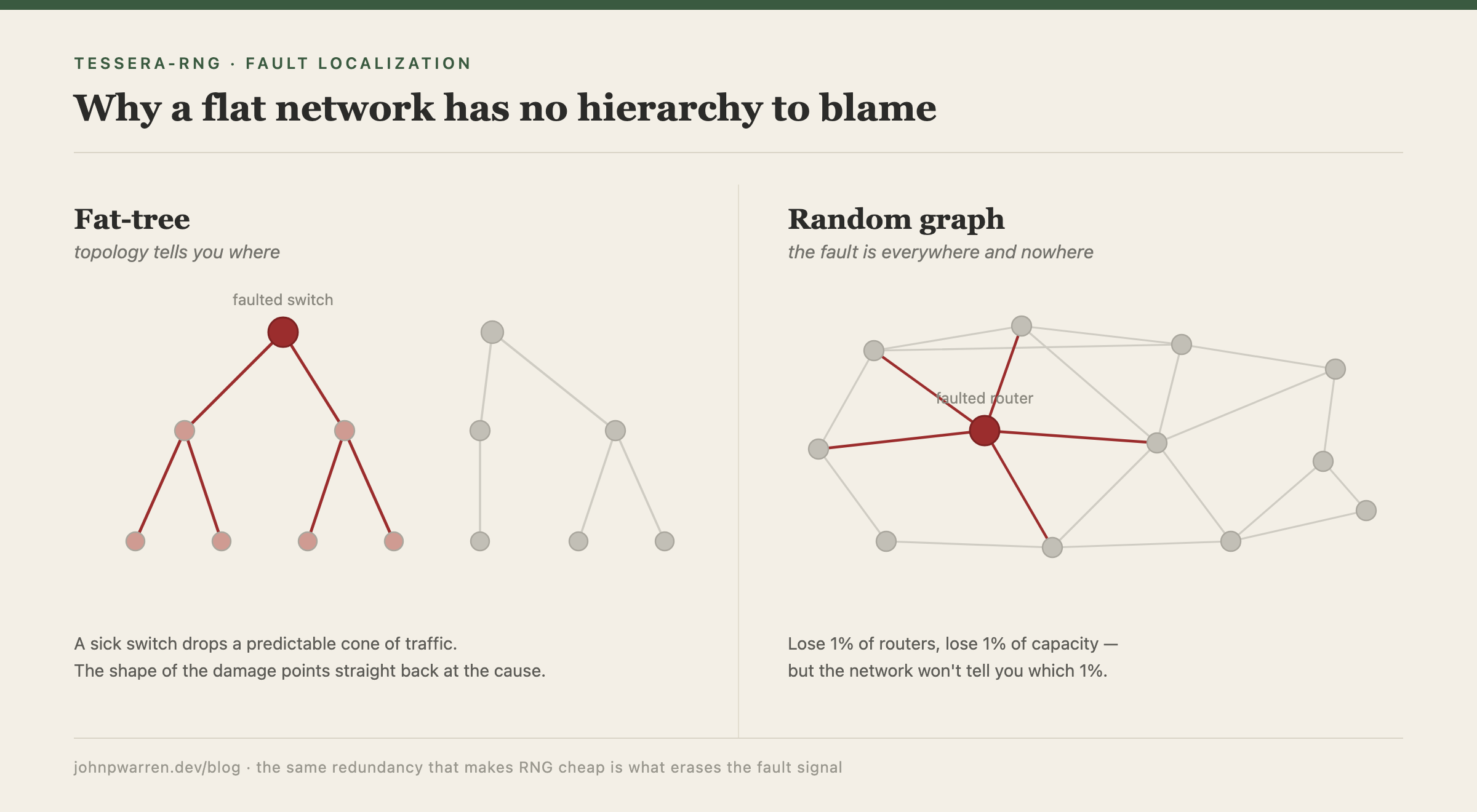
In a fat-tree, the topology is the diagnostic. Hop distance and layer position tell you where a fault lives: a sick spine switch takes down a predictable cone of traffic, and the shape of the damage points back up the hierarchy at the cause. That works because the tree forces traffic through a small number of known choke points.

RNG removes the choke points on purpose. The paper’s structure is a quasi-random expander of degree 64, maximum path length 5, with more than 50 edge-disjoint paths between any endpoint pair, and a forwarding scheme called Spraypoint that sprays each flow across all of them. The property that makes the network cheap and survivable — every pair reachable many ways, no spine left to lose — is the same property that erases the topological signal you would use to find a fault. Lose 1% of routers and you lose 1% of capacity; the network will not tell you which 1%. The paper says so directly, and I confirmed it by reading the construction: hop distance, the thing a tree-shaped monitor leans on, is structurally dead.

So the cheap network ships with one operational bill attached. When something degrades, the topology that used to answer “where” has nothing to say.

The part that transferred for free

Tessera was built for GPU clusters: shard observability across thousands of correlated shards. I took the layer that does the localizing — designed for cluster shards — and pointed it at a network. That layer never relied on hop distance or hierarchy, the cluster’s or the network’s. It localizes to a shared-resource fault domain by watching many monitored entities at once, finding where they stop agreeing, and attributing the disagreement to the physical resource they have in common — a tomographic solver over a fault-domain incidence hypergraph, not a walk over the wiring. None of that asks how many hops apart two things are.

That made the bet cheap to state. Repoint the leaf from “cluster shard” to “network path-class,” repoint the fault domain from “host or rack” to “shuffler, panel, or room,” and the same engine should localize a network fault on a topology where hop distance means nothing. The reusable idea is not the GPU plumbing. It is a bank of statistical detectors that share one alpha budget and hold the false-positive rate at a guaranteed level across however many entities they watch, and that idea does not care whether the entities are shards or path-classes. What Tessera-RNG had to add was the part specific to this problem: a model of the RNG fabric, the per-path-class signal contract, and a tomographic solver that swaps the engine’s hop-distance search for a probabilistic set-cover over the incidence hypergraph. Whether that combination actually localized a fault was the open question.

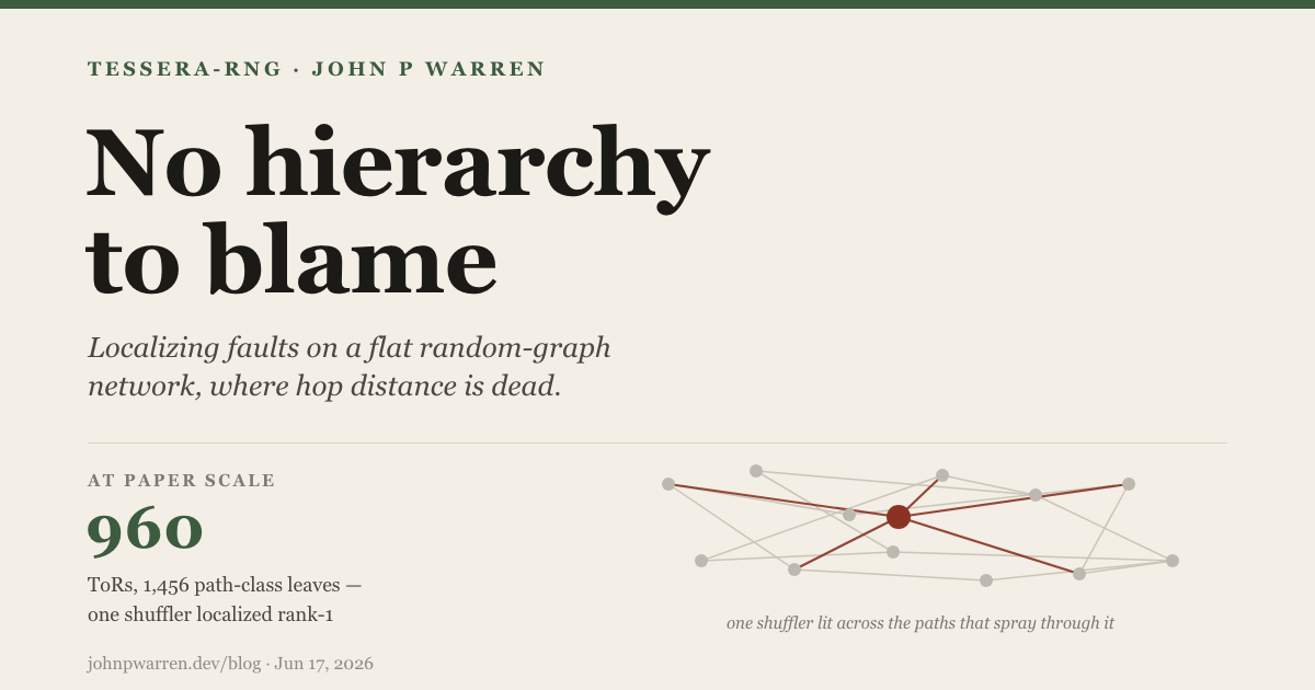
It transferred. On a synthetic fabric built from the paper’s published numbers at full scale — 960 ToRs, about 1,456 monitored path-class leaves, roughly 514,000 weighted incidence edges — a single shuffler driving a common-mode shift ranks first among suspected fault domains, a clean fabric selects nothing under FDR control, and the whole pipeline is byte-identical on replay. The engine’s own hop-distance localizer would have returned noise; the set-cover over physical incidence returns the shuffler.

The detector fires before a threshold would

A path-class emits a handful of signals per tick, and you could read them as a row of dashboards with a red line on each. That reading misses the whole mechanism. A static threshold is a fixed line on one metric, checked each tick on its own: p99 latency crosses forty milliseconds, page someone. It has no memory. A signal drifting steadily toward trouble while every tick stays nominally green never trips it, and two signals that each look fine alone but have stopped moving together never trip it either. At fleet scale the static threshold has no good setting: a line tight enough to catch real shifts pages constantly, and a line loose enough to stay quiet catches nothing.

What ported over from Tessera is a different object. Each signal on each path-class is watched by a betting e-process — an anytime-valid sequential test that bets against the hypothesis that nothing has changed and compounds its winnings tick over tick, accumulating evidence instead of judging each tick in isolation. A slow drift that never crosses a single-tick line still compounds wealth in the process until it fires, and that is the literal content of catching a trend before it crosses a threshold. Because the test is anytime-valid — Ville’s inequality bounds the false-alarm probability no matter how often you look — you can evaluate it every tick. Re-check a static threshold that often and its false-alarm rate climbs with every look; the e-process carries no such penalty.

Two of the detectors see shifts that no per-metric line can. One watches the joint distribution across the signals through a covariance learned from healthy traffic, and fires when they stop co-varying the way the clean fabric taught them to — a correlation flip with every marginal mean and variance unchanged, invisible by construction to any threshold on any single metric. The other watches for periodicity, an oscillation that develops with no change in level or spread at all.

“Normal,” meanwhile, is not one number. The calibration substrate keys a separate baseline to each (hour-of-day, day-of-week, traffic-class) cell and pre-whitens temporal autocorrelation with a per-signal AR(p) model, so a detector compares against the normal for that hour and that traffic rather than a single global line. The fleet layer then combines the per-leaf e-values hierarchically and applies e-BH to control the false-discovery rate at a target q across all 10³ to 10⁴ path-class leaves at once, under arbitrary dependence. The guarantee is on the rate of false discoveries across the whole fleet — and the aggregation into path-classes is what holds the monitored count at thousands rather than the million underlying flows, so the whole thing stays tractable instead of a pager that never stops. One boundary stated plainly: that fleet-level guarantee holds at each query you make, not uniformly over the endless stream. The uniform version is not mine to prove; a 2025 impossibility result (arXiv:2501.04130) shows no streaming procedure with finite detection delay can have nontrivial worst-case FDR.

How well it works, measured

The repo publishes a coverage matrix that is the real answer to “does this work,” so here is its shape rather than an adjective. Magnitudes are in units of the calibrated per-path residual’s standard deviation: Δ=2 means the path-classes crossing the faulted resource shift by about two sigma, before dilution. If sigma isn’t your daily unit: one sigma is a path’s normal tick-to-tick jitter, after the system has accounted for hour of day and traffic class. A 2σ fault moves the average by twice that jitter — obvious in hindsight on a graph, but comfortably inside the range where a static threshold stays green.

condition	measured result
Clean fabric, no fault	0 false selections on both fabrics, and still 0 with realistically contaminated calibration history
Sustained 2σ shift, every fault kind	100% detected, 100% attributed to the correct resource
Two simultaneous 2σ faults	both culprits in the top two, cross-kind and same-kind
1σ shift	detection 25–75%, attribution unreliable; a broad power-zone fault is the exception (100% at 1σ)
0.5σ shift	quiet
Correlation flip / oscillation	floors at Δρ=0.4 and amplitude 0.9, each caught by the detector built for it

The row worth internalizing is the middle one: at two sigma the system names the right physical resource essentially whenever it detects, from a single optic up to a room, at demo scale and spot-checked at 960 ToRs (rank-1 at Δ=4). Between one and two sigma it is a reliable alarm with an unreliable culprit. And when it is pushed past its limits (by noise, missing data, or dilution) it fails by mis-attributing while detection stays green, not by going quiet. That failure mode is why the matrix publishes detection and attribution as parallel columns everywhere: a strong detection rate is never allowed to hide weak localization.

Read the floors as coarse: four runs per cell on a magnitude grid, not re-swept at full scale, all of it synthetic. The matrix is test-bound so the numbers can’t drift from the code. But what a 2σ residual shift means on real hardware depends on the telemetry assumption the next section is about.

The assumptions the paper never published

The transfer rests on two things I should state plainly, because neither appears in the published work. The first is the fabric itself. RNG documents the topology, the routing, the ShuffleBox optics, and the deployment scale, so I rebuilt a fabric from those numbers — 960 ToRs, degree 64, the Spraypoint edge-disjoint path counts — as a synthetic stand-in. It is a simulacrum, not a copy: it reproduces the structure the paper describes, and it may still differ from Amazon’s real network in ways the paper never exposed.

The second is the telemetry, and it is the assumption the whole result rests on. The paper treats operations as out of scope, so there is no published signal contract — nothing that says which per-path-class measurements a real fabric emits. I chose five, one vector per path-class per tick: p99 latency, retransmit rate, loss rate, ECMP imbalance, and path completion — conventional network-health measurements. Two of the five are weaker than they look: ECMP imbalance is topology-specific, and retransmit rate and path completion have the thinnest real-world evidence behind them. The method’s validity does not rest on the signals being exactly these five. It rests on the correlation structure underneath them: when a shared resource degrades, the path-classes that traverse it move together, and the FDR control plus the set-cover invert that co-movement back to the resource. Any telemetry carrying the same co-movement would serve. And the tolerance is now measured rather than assumed: a perturbation study degrades the synthetic telemetry along four axes (noise, missingness, delay, aggregation error) and re-runs the whole stack. Attribution survives half a sigma of uncalibrated noise and 80% missingness before the envelope gives out.

So the honest status is narrow: the math is FDR-controlled and the fault domain is identifiable on a simulacrum of the published fabric, under a telemetry contract that is plausible but unconfirmed. (“Identifiable” is now computed, not asserted: every audit ships a certificate naming any resources the fabric makes indistinguishable; the published fabrics have none.) That is unfalsified, not validated. The one thing that would move it in either direction is a trace from a real fabric — which is exactly what the paper did not publish.

Where the data contradicted me

The parts worth writing down are the places the synthetic fabric refused to agree with my design.

I started multi-fault localization with a binary set-cover that picks the minimal set of fault domains explaining the selected leaves. The first end-to-end test with two simultaneous faults falsified it immediately: the cover claimed a single ToR leaf, reached through a 0.1-weight incidence membership, as the sole culprit for both faults. That is the kind of answer that looks decisive and is wrong. I rebuilt the cover to score candidates by marginal log-likelihood-ratio against the already-picked set, which recovers both faults and reduces exactly to the old scorer at the first pick. The test caught the defect; I did not.

I also drafted the detection and attribution floors before measuring them, and the predictions were wrong twice. A room-level fault that “should” be attributable at the smallest injected magnitude turned out to detect on every seed yet attribute on none of them — the real boundary sits around magnitude 1.5 to 2, not 1. So the published floor reads as a reliable alarm with an unreliable culprit, because that is what the measurement said. I replaced the guesses with the observed numbers and let the uncomfortable one stand. The uncomfortable number has since improved a step (the same fault now attributes on every seed at magnitude 2), and it moved the way it was set: by measurement.

The third was a fuller exposure model I was sure was more correct. I built the full-support variant first and measured it, and it collapsed cross-kind localization: a binary fire-or-quiet scorer drowns when a fault domain touches 63 heavily diluted leaves at weight 1/63. I reverted it and recorded the condition under which it would be worth revisiting (a magnitude-aware member model). Two weeks after this post first went up, that condition was met: the magnitude-aware member model went in, the fuller exposure model went back in with it, and together they are now the production default. Cross-kind faults recover on every seed at every magnitude tested, where the binary scorer recovered none at the high end. (The member model has since been rebuilt once more, into an exact Gaussian model whose null has no parameter a fleet-wide event can corrupt.) Reverting was still the right call. Writing down the revisit condition is what made the return trip cheap.

Two more contradictions arrived after publication, and they belong on this list.

I wrote above that a clean fabric selects nothing under FDR control. That was true and it flattered the system: the calibration window was as short as the test window, so the baselines had never met a realistic week of telemetry. A week-spanning clean run produced 18 false positives, and calibration history contaminated with the clustered aberrations real networks always carry produced 434 across four trials. The fix was structural: every per-cell baseline is now estimated robustly (outlying history is discarded instead of absorbed) over a null that spans the full week. False positives went back to zero in both regimes, at a published cost in clean-data detection floors — four rose a step. The FDR theorem was never wrong. The estimator feeding it was.

The periodicity detector’s guarantee was worse: measurably invalid. Its null assumed a Gaussian statistic that is in fact right-skewed, and the e-process was quietly over-betting: an average wealth multiple of 1.121 per clean window where validity demands at most 1, a 1.3% false-alarm rate against a claimed 1%. It now bets on the rank of the statistic instead, valid by exchangeability with no distributional assumption, and the measured rate sits back under the claim. The invalid over-payment had been buying real detection power below the published floor; that power was given back too, and the floor table says so.

What is left

The localizer cost almost nothing to move from GPUs to a network, because it never depended on which machine it was watching — only that many redundant entities should agree, and a fault domain is wherever they stop. The redundancy that makes a random-graph network cheap is the same redundancy that localization feeds on; the property the paper sells as graceful degradation is, read from the operator’s side, a dense correlation signal waiting to be inverted. The one thing I cannot buy without a live fabric is the five-signal contract the paper left out — the single measurement that would turn “unfalsified” into “validated,” and the only one that would settle whether any of this holds against a real network.