The first five posts in this series were about the AI inference reliability stack: Anchor as the methodology, DeploySignal as the deploy gate, Tessera for steady-state cluster observation, Anvil for chaos-experiment verdicts, Cairn for postmortem attribution. Five projects, one statistical engine, one methodology.

This post is about a different problem domain. Runway is a vendor-neutral, open-source tool for capacity planning of AI compute — answering “when does declared demand outrun deployed capacity, what’s slipping, and what intervention helps most?” Different stakeholders (financial-planning leadership, capacity PMs, service VPs), different math (bootstrap CI + empirical-Bayes slip priors + Monte Carlo runway distributions), different language stack (Python rather than TypeScript), and at v1 a different substrate from the inference-reliability bundle.

What carries forward is the methodology. Anchor from round 1. Anti-scope ledger with v1 hooks. Cold-eye Reviewer cycles. Memorial accretion across projects. The disciplines travel; the substrate doesn’t.

The 2026 context grounds why this tool exists now. The five largest U.S. cloud and tech companies’ aggregate annual AI infrastructure commitment is projected at $660-690 billion in 2026, nearly double 2025. Roughly half of planned U.S. 2026 datacenters are delayed or cancelled; only about a third of the expected 12 GW of new capacity is under active construction. Power and grid permitting have become binding constraints alongside silicon — silicon as the short-term bottleneck, power and grid as the long-term one. Token consumption is forecast to grow ~24× between 2026 and 2030 as agentic workloads scale, while per-token cost drops 60-70% per year — the “cheaper tokens, bigger bills” paradox that has CFOs flying blind on AI infrastructure commitments.

Operators planning AI compute capacity through that environment have been doing it in spreadsheets. Runway is what the spreadsheet would look like if it had been engineered.

The capacity-planning gap

Today’s pattern: capacity teams at hyperscalers, neoclouds, sovereign AI orgs, and large AI labs run capacity-vs-demand calculations in spreadsheets. The spreadsheets get hand-maintained, are brittle to lead-time slips and demand pivots, and produce point estimates that don’t survive a board-level question of the form “how confident are you that we meet Q3 demand?” The answer is usually a verbal “pretty confident” because there’s no calibrated number behind it.

Three things have made the spreadsheet pattern fail specifically under AI workload dynamics:

Token consumption no longer scales with user count. A basic chatbot might use ~200 tokens per session; a multi-step agent that plans, retrieves, invokes tools, reflects, and self-corrects can use 100-1000× that. Workload composition shifts (more agentic, more reasoning-time-compute, more eval runs) produce demand surges that look like the user-count line is exploding when really the per-task multiplier is what changed. Spreadsheets that forecast on “next year’s usage = this year’s × 2” miss this by an order of magnitude.

Power, not just silicon, is binding. Through 2025 the binding constraint shifted from chip allocation to transformers, switchgear, batteries, grid interconnects, and substation upgrades. A planner who has GPUs allocated but a substation upgrade slipping to Q3 has different realistic capacity than a planner whose GPU allocation matches the power delivery curve. Modeling “GPUs available at date X” without modeling “power delivered to those GPUs at date X” produces optimistic plans that fail at integration time.

Supplier promises slip at industry-known rates. With about half of planned 2026 buildouts delayed or cancelled, the base rate for “the supplier will deliver what they committed to” is roughly 50%. Plans built on point-estimates of committed delivery dates ignore the most important variance in the entire system. Capacity teams know this intuitively but their spreadsheets don’t.

The narrower question Runway answers, with these dynamics taken seriously: given declared demand history with a growth model, committed supply with stage-level slip risk, power-delivery constraints, and intervention options (expedite OEM, pull-in onsite, shift demand, lift MFU (model-FLOPs utilization), add buildorders, upgrade power), when does demand outrun realistic capacity, what’s the dominant slip contributor, and which intervention buys the most runway per dollar?

The audience is the VP/SVP of Compute (supply-side capacity owner — runway date, what’s slipping, where to intervene) and the financial planner / CFO who needs to defend the capex spend to the board. Same engine, two different views of the same numbers.

The statistical core

Five load-bearing pieces.

Demand forecasting with bootstrap CI. Three growth models — exponential, linear, piecewise — fit via OLS in log-space (exponential) or linear-space, with residuals bootstrap-resampled (1,000 replicates, seeded by (scenario.name, sku) for reproducibility) to produce 80% and 95% confidence bands. Bootstrap is the right choice rather than parametric CI because GenAI demand series are short, non-normal, and prone to regime shifts; empirical residual resampling captures that without assuming a distribution. Piecewise mode fits slope from a recent window only, anchored to the last observed point — captures regime shifts (launch events, demand pivots) without the pre-shift trend dragging the extrapolation.

Stage-level slip propagation. Build orders are modeled as ordered stages (OEM → supplier → onsite, recommended; arbitrary kinds supported). Slip propagates: a stage can’t start before its predecessor ends, even if its planned_start was earlier. Per-vendor empirical-Bayes priors shrink toward the overall fleet mean when vendor-specific history is sparse — operators with little internal history still get reasonable priors. Industry-grounded slip-rate priors are landing as a v2 add, bundling the ~50% base rate from public datacenter-delay reporting so operators with no internal data at all get defensible starting points.

Binding-constraint detection (chips vs MW). BuildOrder.power_per_unit_mw + Scenario.power_capacity_mw (or regional_power_capacity_mw) let the engine compute the binding constraint at each point in the horizon. The RunwayResult.binding_constraint field reports "chips", "power", or "none" — surfacing whether the operator’s plan is gated by GPU availability or by grid-side delivery. Power-aware optimization treats power-upgrade interventions (substation work, feeder upgrades) as deltas at $1.5M/MW default for hyperscaler-grade — so the optimizer considers MW capacity upgrades alongside chip expedites.

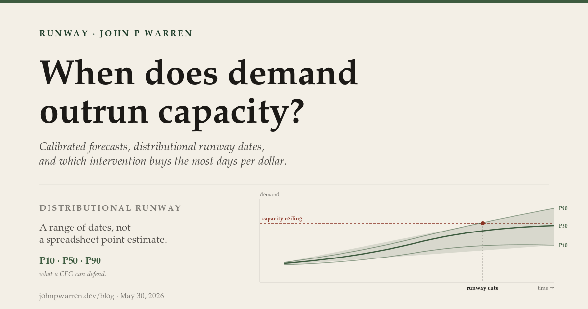
Monte Carlo runway distribution. The point-estimate runway date is one number; the operator needs a distribution. Monte Carlo perturbs demand growth rates, per-stage slip realizations, and MFU drift across N runs (default 200) and returns the runway date distribution: P10 / P50 / P90 plus a CDF. The output is a probabilistic answer to “when does demand outrun capacity” — operator gets back not a date but a range of dates with explicit probability weight, which is what a CFO needs to defend a capex decision.

Sensitivity analysis and backtesting. A tornado chart shows which parameters move the runway date most: demand growth, stage slip, MFU, availability factor, power capacity. Operators see at a glance which input assumption their forecast is most sensitive to. Backtesting replays forecasts as-of historical dates and compares to actuals, returning MAPE (mean absolute percentage error), 80%/95% confidence-interval calibration, and predicted-vs-actual runway error — so the calibration claim isn’t taken on faith.

Worked example. The Hyperscaler 2027 scenario shipped with the package: 10 AWS-style regions × 4 SKUs (H200, B200, Trainium2, A100) × 36 months of history × ~60 build orders × 36-month horizon. $39.9B total capex. Realistic at-Amazon scale. The engine produces per-region runway, per-SKU runway, per-service runway (Bedrock / SageMaker / internal-retail-genai split), capex pacing waterfall, supplier scorecards, and a Pareto frontier of intervention cost vs. runway improvement — all from one engine pass, all deterministic and replay-clean.

The audit log records every scenario load, API call, export, anomaly, and threshold-crossing event, with JSONL persistence available. Same compiled inputs produce the same outputs, byte-identical. Same property as the DeploySignal audit substrate — a board-deck PDF can be re-derived from first principles months after the fact.

Multi-stakeholder views as the differentiator

The most underserved part of the capacity-planning gap isn’t the math — it’s that nobody has built a tool that surfaces the same engine to the operator AND the finance team AND the executive in views they each need. The current state is operators run their spreadsheet, finance runs their FP&A model, the CEO sees a quarterly slide. Three disconnected sources, one set of underlying numbers, no shared substrate.

Runway ships four stakeholder views over one engine:

• Capacity PM page. Supplier scorecards, per-order detail, slip predictions per (vendor, kind) under the empirical-Bayes prior. This is the operator’s working surface — where the day-to-day capacity decisions are made.
• Service-VP page. Per-service runway (Bedrock, SageMaker, internal-retail-genai, etc.), per-tenant demand attribution, SLA-tier breakdown (platinum / gold / standard), locality-binding warnings when a workload’s regulatory or latency constraints leave it short of capacity in its allowed regions. The service owner sees their slice without the noise of the rest of the portfolio.
• CFO page. Capex pacing waterfall (committed vs. delivered dollars over time), unit economics ($/token, $/query, $/training-hour), net-present-value comparison across Build / Lease / Reserve strategies (operator-supplied cost of capital, lease rate, reservation discount, depreciation years), board-deck PDF export.
• CEO page. Single-pane R/Y/G summary of runway status across regions and SKUs, PDF export, one number with one CI band.

Same engine. Different surfaces. The defensibility argument lives in the fact that the CFO and the operator are looking at the same underlying numbers — the CFO’s $/token doesn’t disagree with the operator’s runway date because they’re computed from the same compiled scenario, with the same audit trail, on the same deterministic engine.

This is what spreadsheets structurally cannot do. A spreadsheet built for the operator gets a copy-paste relationship to the CFO model and they drift. Runway’s two-layer architecture (runway_core engine + runway_app UI) keeps every view a thin projection of one source of truth.

Methodology

Runway was built using Anchor from round 1, same pattern as Tessera. v1 — fourteen minor versions, v0.1 through v0.14 — shipped in a single day. v0.15, the v2 batch, shipped the next day with five more load-bearing capabilities (covered below). Both days applied the same Wave-Plan / Q-Plan / Reviewer-cycle discipline per version. The CHANGELOG documents the round-by-round progression: each version a discrete capability set, each shipped behind cold-eye Reviewer audit, each preserving prior anti-scope hooks.

The discipline that made fast shipping safe is the anti-scope ledger with v1 hooks. From SCOPING-MEMO §7: every anti-scope item (multi-SKU portfolios, DAG-parallel stages, confidence-weighted ensembles, real $ cost optimization, live data connectors, non-GPU units, sub-monthly granularity, custom stage kinds, user-defined delta types, hosted multi-tenant deployment, auth/RBAC, Pandas→Polars migration) has an explicit v1 design hook so the future-extension door stays open. Twelve items, twelve hooks. The discipline asks for each: is there a v1 hook that makes v2 additive rather than rewrite? The one acknowledged one-way risk (Pandas → Polars/DuckDB) was explicitly flagged as such and mitigated by v1 dataset sizes being orders of magnitude below the threshold where it matters.

The cross-project memorial brought inherited disciplines from the inference-reliability bundle forward. Audit-substrate continuity, deterministic engine outputs, replay-clean records, ESCALATE patterns for spec/reality mismatches, anti-self-confirming-tests check at every assertion — none of these had to be discovered for Runway because they were already memorialized from DS and Tessera. DeploySignal’s v1 took four weeks. Runway’s took one day. The cost of starting Runway was lower than the cost of starting DeploySignal by exactly the amount of accumulated discipline.

This is the compounding claim from the Anchor post showing up in a different problem domain. The methodology travels into a project whose substrate is fundamentally different — Python instead of TypeScript, capacity planning instead of statistical detection, finance-facing stakeholders instead of SRE-facing — and the disciplines still apply. That’s what general in “general-purpose methodology” was supposed to mean.

The Tessera adapter

Runway v1 was deliberately independent of the inference-reliability bundle. The SCOPING-MEMO carved this out explicitly: no shared engine or data dependency at v1; future intersection points (e.g., Tessera utilization signals → Runway demand calibration) noted as v3+ and out of scope. The carve-out preserved Runway’s adoptability — orgs without DS or Tessera installed can still use Runway as a standalone capacity planning tool.

v0.15 brought that intersection point forward. runway_core.adapters.tessera.TesseraAdapter consumes Tessera’s TesseraToDsFeedRequest wire format — but reads it from JSONL replay files or dict iterables rather than via an HTTP call to a running Tessera instance. The decoupling is deliberate: orgs that run both can pipe Tessera’s audit JSONL into Runway with a cron job; orgs that don’t run Tessera ignore the adapter entirely. No runtime dependency either direction. Adoptability preserved.

The adapter filters to cluster_event_id == 'capacity_change' (the other four event classes — firmware_push, model_redeploy, env_change, config_change — are deploy-side and already handled by Tessera’s freeze-hook). Capacity-relevant VerdictGroups aggregate into monthly CapacityPressureSignal events per region with α-weighted pressure scores. anomaly.detect_anomalies(..., capacity_pressure_signals=...) escalates severity by one level when a forecast/actuals divergence AND a Tessera signal point the same direction. The output carries dual-source citation (sources=['forecast_divergence', 'tessera_capacity_pressure']).

Single adapter, not two. The DS↔Tessera coordination contracts handle the deploy-event suppression layer internally to the bundle — Tessera knows about deploy windows via the cluster_event_id field, including the capacity_change event class that’s signal-worthy rather than suppression-worthy. Downstream consumers (Runway, Cairn) join the established pattern of consuming Tessera’s outbound surface, not separately integrating with each upstream product.

What this composition produces: when production telemetry diverges from the declared demand series, Runway sees it through Tessera before the operator notices it on a dashboard. The runway date updates with citation back to specific Tessera VerdictGroups. The forecast becomes self-calibrating against production reality in a defensible way — operator gets back not “the runway moved” but “the runway moved 12 days because Tessera Family A and Family C fired sustained-pressure patterns on rack-7 over the last 9 days, and the demand series you declared is undershooting actuals by ~8%.”

The lifecycle frame extends one more time. DeploySignal catches before promotion. Anvil verifies under chaos. Tessera observes during steady state. Cairn attributes when something escapes them all. Runway plans forward, calibrated by Tessera’s observations. Five operational questions, one shared statistical engine for the first four, a separate substrate for the fifth — and the methodology covers all of it.

v0.15: closing the 2026 gap list

The day after v0.14, v0.15 shipped four more capabilities (alongside the Tessera adapter covered above) matching the gaps the 2026 capacity-planning discourse calls out:

• Agentic compute distributions. WorkloadDemand.compute_distribution accepts a PointCompute, GaussianCompute, or MixtureCompute (named components with weights). Captures the multi-step-agent multiplier and the reasoning-depth-variance pattern in one abstraction — same root cause both ways, per-task compute is a distribution not a point. Distribution variance propagates additively into bootstrap demand confidence intervals, which widen realistically when mixture components have wildly different per-task costs. The “cheaper tokens, bigger bills” paradox becomes modelable without operators inflating growth rates by hand.
• Industry-grounded slip priors. data/public_slip_priors.yaml ships four stage-kind priors (oem_chip_delivery, onsite_buildout, power_substation, supplier_general) with citations to public sources (FERC interconnect queue, Deloitte AI Infrastructure 2026, SemiAnalysis). The empirical-Bayes slip predictor shrinks toward the matching prior when a vendor has fewer than three historical orders — so operators with no internal history still get defensible starting points.
• Power as a delivery curve. A new PowerDelivery model with stages mirroring BuildOrder.stages lets scenarios model substation work, grid upgrades, and interconnect permits as time-series deliveries with their own slip risk. power_capacity_curve_mw returns MW availability over the horizon; the binding_constraint logic now surfaces realistic mid-horizon transitions (“you have H200s in May, your substation upgrade ships in July, so realistic capacity is X through July not Y”).
• Eval as a first-class workload kind. WorkloadDemand.kind = "eval" plus three eval-specific sizing fields: eval_model_size_params, eval_cadence_per_month, eval_compute_per_param_per_run. Total compute = params × cadence × compute_per_param_per_run. Eval workloads, often invisible in capacity plans, become distinct rows in the TCO breakdown.

All additive against existing v1 anti-scope hooks. No rewrites.

Close

What this post closes, alongside Cairn closing the inference-reliability series, is the deep-dive cadence for the projects that exist. Five products in the inference-reliability bundle plus Runway makes six. The next posts in this series will get to whatever ships next, when it ships in a state worth deep-diving on.

The arc the six posts trace together: build the inference-reliability stack, distill the methodology along the way, codify it as Anchor, apply it from round 1 to a project in a different problem domain. The methodology travels. The substrate doesn’t. That’s the design.